The Auxiliary Field
Last time (before break):
The “Gilbert” model:
You can do a lot of magnetostatic problems by using electrostatic results and replacing:
- \(\vec{p}\) with \(\vec{m}\)
- \(1/\epsilon_0\) with \(\mu_0\)
- \(E\) with \(B\)
Once you get really close-up to the dipole (where it looks like a ring of current instead of a perfect magnetic dipole) then this breaks down. Griffiths’ advice is to use the Gilbert model to get intuition, but don’t rely on it for quantitative results.
Paramagnetism
A magnetic field will polarize matter. It will change its magnetic moment by:
\[\Delta \vec{m} = -\frac{e^2R^2}{4m_e}\vec{B}\]where \(R\) is the radius of the “orbit” of the electron.
Notice the change in \(\vec{m}\) is opposite the direction of \(\vec{B}\).
\(\vec{M}\) is the magnetic dipole moment per unit volume (just like \(\vec{P}\) is the electric dipole moment per unit volume.)
In polarized matter we calculated a bound charge (both volume and surface.) In the same way for magnetized matter we can calculate bound current (both volume and surface.)
The idea of bound current and bound charge give you a way to think about why the field is changed by the material, but it’s not a good way to calculate the field (not usually, anyway).
Today - Auxiliary Field
Today Dave is going to tell you about the auxilliary field \(H\) which is the better way to calculate the field in magnetized matter.
The Auxiliary Field
Just like we did with electric charge, we can do with current. To calculate the magnetic field we can consider the free current density \(\vec{J}_f\) and the bound current density \(\vec{J}_b\). The bound current density is really sort of an “effective” current density due to all the electronic orbits in the matter. For the sake of calculating the electric field, you need to consider it.
\[\vec{J} = \vec{J}_b + \vec{J}_f\]Griffiths makes the point here that this is NO NEW physics. It’s really just saying “Magnetization effectively adds current, and you have to include that current when you’re calculating the field.”
So then we can use Ampere’s law as before:
\[\frac{1}{\mu_0} (\nabla \times \vec{B}) = \vec{J}_b + \vec{J}_f = \vec{J}_f + (\nabla \times \vec{M})\]As we did with electric fields we bring all the \(\nabla\)’s over to one side…
\[\nabla \times \left( \frac{1}{\mu_0} \vec{B} - \vec{M}\right) = \vec{J}_f\]And you know (from what we did with \(\vec{E}\) and \(\vec{D}\) that I’m about to tell you that the thing in parentheses is \(\vec{H}\), but before we say that, let’s remind ourselves what we just did…
The \(\vec{B}\) in the equation just above is the TOTAL \(\vec{B}\), due to the free current and the bound current added together. We subtract off the piece due to the magnetization. What’s left is the piece that’s due to the free current. So what I’m about to call \(\vec{H}\) is really the field ** NOWHERE**. It’s not a physical quantity. It’s just way more useful for doing problems than calculating bound currents.
Having said all that I will say:
\[\vec{H} = \frac{1}{\mu_0} \vec{B} - \vec{M}\]and Ampere’s law now reads:
\[\nabla \times \vec{H} = \vec{J}_f\]or in integral form:
\[\oint \vec{H}\cdot d\vec{l} = I_{free}\]Caveat to my going on and on about how \(\vec{H}\) is not a physical quantity
I still stand by my statement. However, Griffiths has a really interesting paragraph (pg 281-282) about how useful \(\vec{H}\) is in the lab. It’s useful because free current is actually the thing you can measure and control, so \(\vec{H}\) is the thing you can control (even though it doesn’t exist.)
Let’s do a problem with it:
Problem 6.12b in the book:
An infinitely long cylinder, of radius \(R\), carries a “frozen-in” magnetization, parallel to the axis,
\[M = ks \hat{z}\]where \(k\) is a constant and \(s\) is the distance from the axis. There is no free current anywhere. Find the magnetic field inside and outside the cylinder. (Use Ampere’s law to find \(\vec{H}\), and then get \(\vec{B}\).)
Reminder: the magnetic field outside a solenoid is zero, and points completely along the axis of the solenoid. Its direction is given by the right-hand-rule.
(Please suggest that they work on this in their usual working groups. They will use all the board space. While they’re working, you should walk around and give hints. If you see someone calculating J or K, gently suggest that H gives you a way of avoiding that completely, which is the point of this exercise.)
Answer:
Use the Amperian loop shown (shaded) in the figure.
If you sketch this figure on the board, leave out the J and K, because their
directions should be a surprise.
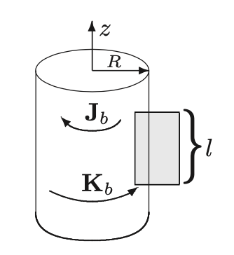
By symmetry, H points in the z direction. Integrating around the Amperian loop gives
\[\oint \vec{H}\cdot d\vec{l} = Hl =I_{free, enc} = 0\]since there is no free current there.
So \(\vec{H}=0\),and hence \(\vec{B}=\mu_0\vec{M}\). Outside \(M=0\),so \(B=0\); inside \(M=ks\hat{z}\), so \(\vec{B} = \mu_0 ks\hat{z}\).
What’s your intuition here for what’s happening?
Ans:
Now I want you to actually calculate the bound current to see if it helps you figure out what is happening.
Ans:
\[\vec{J}_b =\nabla \times \vec{M} =−k\hat{\phi}\] \[\vec{K}_b =\vec{M}\times \hat{n} =kR\hat{\phi}.\]The wikipedia page on Maxwell’s Equations is shockingly useful: Here’s a figure from it:
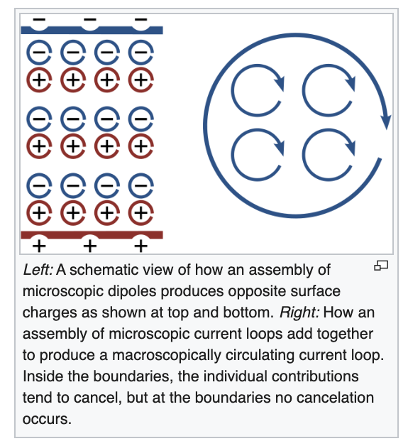
I think this cartoon does a good job of explaining the direction of the surface current, \(\vec{K}\) which is in the same direction (by the right-hand rule) as the magnetization.
How do you explain the volume current going in the opposite direction???? I think I can explain it by virtue of the magnetization increasing with \(s\). You can expect the little current loops to cancel out completely if one is bigger than the other. And if the inner one is smaller than the outer one then the part that ends up not cancelling will be going in the opposite direction as the current loops.
Boundary Conditions
(I don’t actually think we’ll get a chance to talk about these in class, but I put them here for reference.)
The boundary conditions on \(\vec{H}\) are:
\[H_{above}^\perp - H_{below}^\perp = M_{above}^\perp - M_{below}^\perp\] \[\vec{H}_{above}^\| - \vec{H}_{below}^\| = \vec{K}_f \times \hat{n}\](Notice that the perpendicular boundary conditions are not vectors, because \(\vec{H}_\perp\) is only one direction, but \(\vec{H}_\|\) is a vector in two dimensions.)